
Below are some example data visualizations that I have created. These are just quick projects to look at something I’m interested in or to explore making different kinds of figures.
What limits river light environments?#
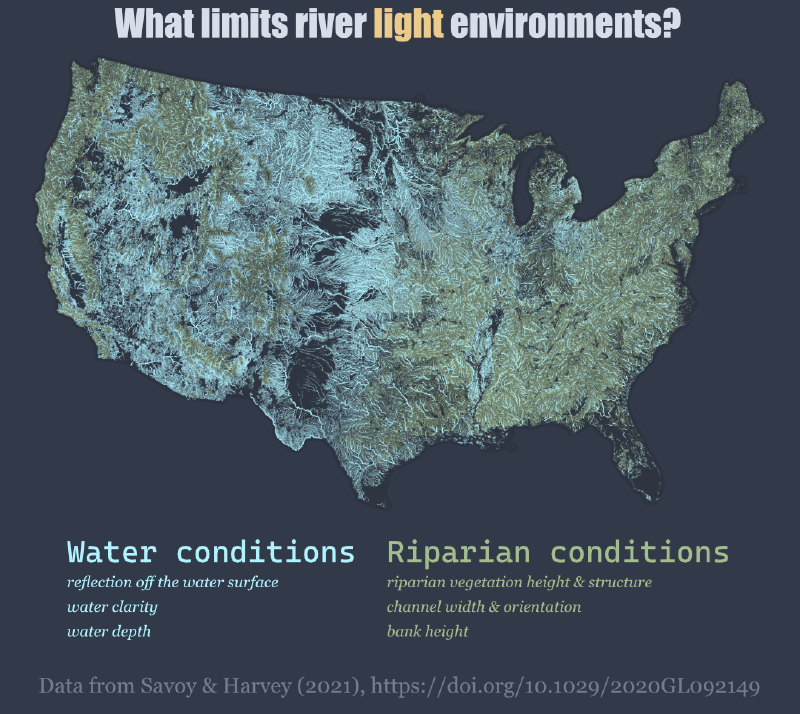
The conversion of solar energy to chemical energy by primary producers is a fundamental piece of carbon cycling and energy flow within ecosystems, but river autotrophs often only receive a small fraction of incoming sunlight. Lighting conditions within rivers are influenced by many factors including the size and shape of the river itself, surrounding riparian zones, and changing water conditions.
A few years ago, I designed a model predict light available for river primary producers and used the model to infer whether productivity was most limited by riparian zones or water column processes for over 2 million reaches in the US. We found that water column processes most limited productivity for 50% of the nation’s river length and 80% of its surface area. At the time we found some variations across the country that appeared to be driven by forest cover, but I thought it would be interesting to visualize predictions using national hydrography flowlines. This was a fun exercise to revisit some old work and look at it in a new way.
If you are interested in learning more about this model or our results, you can find our paper here https://doi.org/10.1029/2020GL092149
Which month has the highest streamflow?#
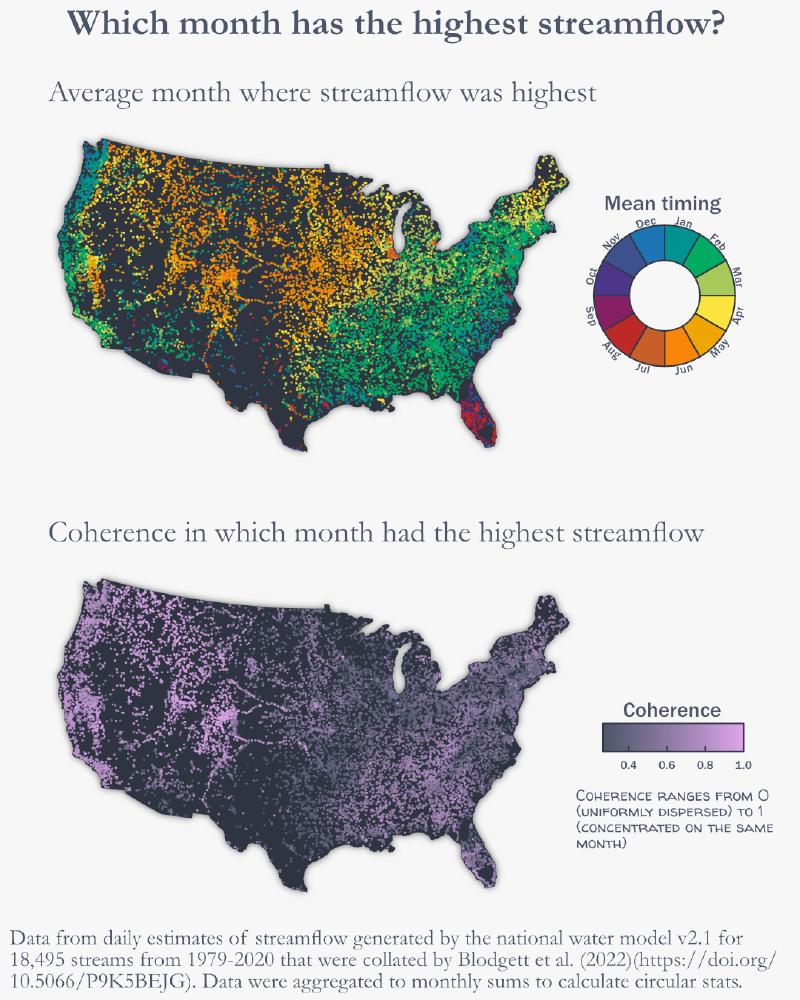
Which month has the highest streamflow? I used retrospective estimates of streamflow from the national water model for 18,495 U.S. streams spanning 1979-2020 to visualize this question. Since modeled streamflow was used, I calculated all circular statistics based on total monthly streamflow instead of using daily estimates.
If you are interested in this kind of analysis using observed data, I would highly suggest reading Villarini (2016).
Where are USGS instantaneous stream water quality sites located?#
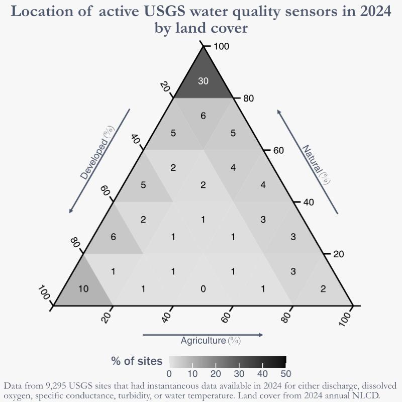
I looked at all active CONUS NWIS sites in 2024 that were recording common water quality measures (discharge, dissolved oxygen, specific conductance, turbidity, water temperature) to see what the surrounding land cover was. 46% of sites were situated in areas where natural land cover was the dominant (>=60 %) class. By contrast, only 9% of sites were located where agriculture was the dominant class.
If you are interested in a deep dive into global bias of stream gauge locations, check out Krabbenhoft et al. (2022) for an excellent analysis.
Terrestrial phenology and stream metabolism#
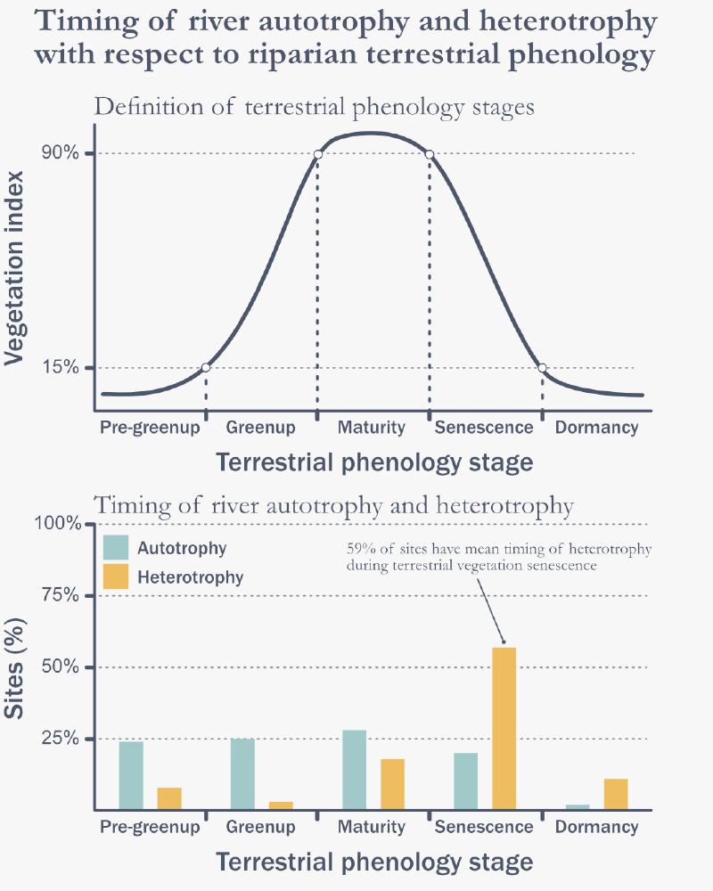
Previously I explored the timing of river autotrophy and heterotrophy by calculating the mean timing of each for a few hundred rivers. Autotrophy more commonly occurred in spring and summer whereas heterotrophy more commonly occurred in summer and autumn. Since terrestrial systems can serve as sources of organic matter inputs to rivers, I wanted to look at the patterns of river metabolism in relation to changes in terrestrial vegetation phenology.
I used MODIS vegetation dynamics data to get stages of terrestrial phenological development at each site (e.g. greenup or senescence) and determined which stage of development autotrophy and heterotrophy occurred in.
Autotrophy was relatively evenly distributed throughout phenological stages, with about 25% of sites falling into each stage outside of dormancy. By contrast, 59% of sites had their mean timing of heterotrophy occur during senescence. The prevalence of heterotrophy during senescence of terrestrial vegetation could be due to inputs of organic matter in the form of leaf litterfall.
If this topic interests you, Bertuzzo et al. (2022) has a modeling study that looks into different sources of organic matter and river ecosystem respiration rates.
Timing of river autotrophy and heterotrophy#
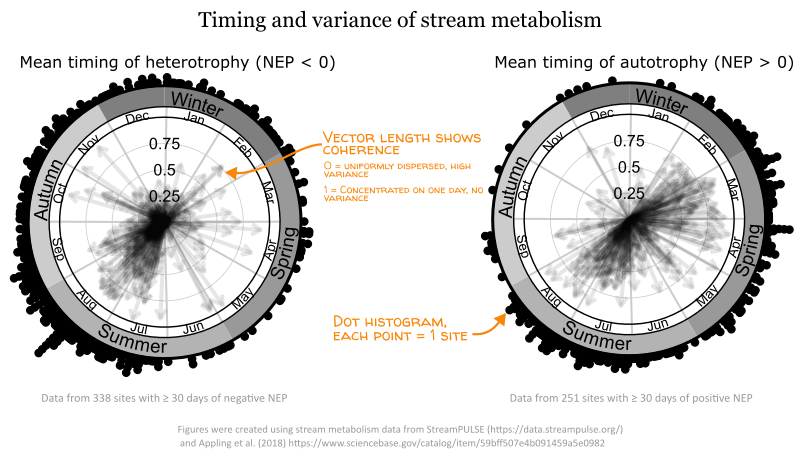
River ecosystem metabolism is useful for understanding energetics and carbon cycling in flowing waters. Net ecosystem production (NEP) provides information on whether a river is autotrophic (NEP > 0) or heterotrophic (NEP < 0) and carbon dynamics within the ecosystem. Are there any consistent patterns in the timing of autotrophy or heterotrophy?
I used circular statistics to calculate the mean timing of days with positive or negative NEP for a few hundred rivers. Additionally, the coherence (or dispersion) was also calculated to see if the timing of these events was concentrated in a specific time of year for each site.
A total of 44% of sites had a mean timing of autotrophy in summer and another 38% in spring. By contrast, 40% of sites had a mean timing of heterotrophy in summer and 37% in autumn. While summer has high percentages of both autotrophy and heterotrophy, it appears that positive NEP is more likely to happen in the spring and negative NEP in the autumn. This is a simple conclusion in agreement with conceptual understanding of biogeochemical cycling, but useful to see it so clearly highlighted in the data.